Let $E\subset \mathbb{R}^2$ be a Borel set with $\mathcal{H}^1(E)<\infty$. The lower density of $E$ at a point $x$ is
\[\Theta^1_*(E,x)=\liminf_{r\downarrow 0}\frac{\mathcal{H}^1(E\cap B(x,r))}{2r},\]normalized by the diameter $2r$ rather than by $r$, so that a straight segment has density $1$ at its interior points.
Question: How large does the lower density have to be, at almost every point, before $E$ is forced to be countably $1$-rectifiable?
Before saying anything about the answer, I want to explain why $1/2$ is the number one should guess. Take the simplest rectifiable set there is: a closed line segment sitting inside $\mathbb{R}^2$. At an interior point $x$, a small ball $B(x,r)$ meets the segment in a piece of length exactly $2r$, so the density is $1$. But at an endpoint, the ball only sees one side, the piece has length $r$, and the density is exactly
\[\frac{r}{2r}=\frac12 .\]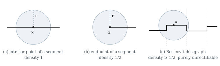
So $1/2$ is what you get from a set that, at every scale, looks like a segment with your point at the end of it. That is the cheapest way to keep the density up while refusing to look like a line through $x$: reach out in one direction only. And this is not a fantasy — Besicovitch’s 1938 example is a purely unrectifiable set of finite length which does exactly this at almost every point, and therefore has lower density at least $1/2$ almost everywhere. So no threshold at or below $1/2$ can force rectifiability, and the guess is that everything above $1/2$ does.
Besicovitch’s 1/2-conjecture: if $\mathcal{H}^1(E)<\infty$ and $\Theta^1_*(E,x)>1/2$ for $\mathcal{H}^1$-almost every $x\in E$, then $E$ is countably $1$-rectifiable.
It is convenient to package this as a single number. Let
\[\sigma_1(\mathbb{R}^2)=\inf\{\beta\ge 0:\ \Theta^1_*\ge\beta \text{ a.e. forces countable } 1\text{-rectifiability}\},\]so that the conjecture reads $\sigma_1(\mathbb{R}^2)=1/2$. The history of the upper bound is a slow descent:
| year | bound | |
|---|---|---|
| 1928 | $1-10^{-2576}$ | Besicovitch |
| 1938 | $3/4$ | Besicovitch |
| 1992 | $(2+\sqrt{46})/12=0.73186\ldots$ | Preiss and Tišer |
| 1998 | $0.72655\ldots$ | Schechter |
| 2024 | $0.7$ | De Lellis, Glaudo, Massaccesi and Vittone |
The $1992$ bound stood for more than thirty years. What I want to report here is one more step:
Theorem: $\sigma_1(\mathbb{R}^2)\le \dfrac{6934}{10000}=0.6934.$
Together with a formalized version of Besicovitch’s classical example, this pins the threshold to
\[\tfrac12\ \le\ \sigma_1(\mathbb{R}^2)\ \le\ 0.6934 .\]Both inequalities are machine-checked. The proof term is complete Lean 4, it contains no sorry, and it depends on exactly the three axioms propext, Classical.choice and Quot.sound — no native_decide, no floating point, no hash, no external oracle. Everything is at github.com/CoolRmal/Besicovitchs-1-2, together with a short write-up of the argument.
The rest of this post is in two parts. The first is about how it was made, which I think is at least as interesting as the result, and the second is about the mathematics.
Part I: how this was actually done
Two stages, two tools
The work split cleanly into a mathematical stage and a formalization stage, and I used different tools for each.
The mathematics was done first, entirely in conversation, in a ChatGPT project, over six days (26–31 August 2026). I did not write Lean during this period at all. What came out of it was $246$ markdown research notes — about $618{,}000$ words — plus $86$ C++ search programs, $16$ LaTeX write-ups and $53$ Python verifiers. Most of it is scaffolding and dead ends. The part that survived is a single document: an argument that reduces the whole problem to thirty explicit rational certificates, together with two independent programs that check them.
The second stage was the Lean development, written by an agent in Claude Code against Mathlib, with me directing the scope. This is the part where I can give real numbers, because the session transcripts record them.
| Phase 1 (abandoned) | Phase 2 (delivered) | |
|---|---|---|
| wall clock | 14 h 54 m | ~5 h for the delivered proof |
| output tokens | $1{,}963{,}539$ | $2{,}512{,}213$ |
| surviving lines of Lean | $0$ | all of it |
Phase 1 spent $94\%$ of the non-cached tokens and $75\%$ of the wall clock chasing the sharp constant through six-variable Bernstein certificates. It produced $24{,}274$ lines of Lean, all of which I deleted. Phase 2 produced the entire delivered proof for about $2.7$ million tokens in five hours.
I think this is the most useful thing in the whole project to report. The two phases differed only in which mathematical argument I handed the agent. Having the right argument was worth roughly a factor of seventeen in tokens, and the difference between “incomplete after fifteen hours” and “done in five”. The bottleneck was never the Lean.
The finished development is about $27{,}000$ lines across $99$ files. The Gram-certificate proof proper — everything the analytic heart of the argument needs — is four files and $1{,}548$ lines. Checking the whole thing from a warm Mathlib cache takes $2$ m $32$ s of wall clock.
Palomar, and what a comparator is for
I submitted the result to Palomar, a registry of Lean-verified mathematics incubated by the Lean FRO and ICARM, announced by Terence Tao in August. The idea is to be the analogue of a preprint server, but for Lean proofs: you submit a repository at a fixed commit, and the registry records what has actually been verified.
The mechanism I found genuinely clever is the comparator. A submission has two Lean modules. Challenge.lean contains the definitions and the statements you claim, with the proofs replaced by holes. Solution.lean contains the same statements, proved. The comparator checks that the solution really does prove exactly the statements advertised in the challenge — not a weakened variant, not a different-looking definition that happens to have the same name.
This addresses the failure mode that worries me most about machine-checked mathematics. A wrong proof cannot get past Lean. But a proof of the wrong theorem can get past Lean easily, and a definition that has quietly drifted is very hard to notice inside twenty-seven thousand lines. In my comparator.json I deliberately did not use the definition_names escape hatch, which means every definition reachable from the statement is compared recursively: sigmaOne cannot be restated or weakened on the solution side.
That leaves exactly one thing a human still has to check by hand, and it is the challenge file. So I checked it by hand. That is a realistic thing to ask of a person: Challenge.lean is about eighty lines. It contains four definitions — lower density, countable $1$-rectifiability, “$\beta$ forces rectifiability”, and $\sigma_1$ as an infimum — and three statements. I read it line by line, more than once, and I would encourage anyone reading a formalization to do the same and ignore the rest.
One thing that check caught, incidentally: Lean’s sInf of an empty set of reals is $0$, so an upper bound on $\sigma_1$ could in principle hold vacuously. That is why the repository also proves $1/2\le\sigma_1(\mathbb{R}^2)$ and compares it alongside, and why it proves separately that every $\beta>0.6934$ really is an admissible threshold. The bound is not vacuous, and now that is a theorem rather than a remark.
On luck
I want to be honest about the role of luck here, because I think the honest version is more useful than either the modest or the immodest one.
This result is, to a large extent, lucky. The six-point problem happened to be the right size: small enough that a finite certificate family could close it, large enough to beat the record. The Gram-matrix argument that made the certificates cheap arrived on the fifth day and could easily not have arrived at all. I had already spent fifteen hours of agent time on a route that turned out to be a dead end, and if the second route had not appeared I would have nothing to report.
But the luck had somewhere to land. I have spent a long time reading around this problem — Besicovitch’s original papers, Preiss and Tišer, the recent linear-programming paper, the standard geometric measure theory. When the Gram argument appeared I recognized immediately what it was worth, and more importantly I could tell which of the many plausible-looking suggestions I received were actually nonsense. That judgment is not something the tools supplied. Most of what came out of six days of conversation was wrong or useless; the value was in being able to say so quickly.
Part II: the mathematics
A classical theorem, and what a quantitative version should look like
Here is a theorem that has been known for a long time.
Theorem (Eilenberg–Harrold): a compact connected subset of $\mathbb{R}^2$ with finite $\mathcal{H}^1$ measure is $1$-rectifiable; in fact it admits a Lipschitz parametrization.
This is the reason connectedness and finite length together are such a strong hypothesis, and it is formalized in the repository because the proof needs it. The trouble is that a set with high density need not be connected at all. So one wants a quantitative substitute: some condition saying that the set cannot be split into two pieces cleanly, which high density might plausibly supply, and which is enough to run the same conclusion.
That substitute is the Besicovitch pair condition. Roughly: whenever you have two measurable pieces $E_1,E_2$ at small positive distance from each other, both of which have density above $\beta$ at all small scales, there must be an open set $V$ meeting both of them which carries a definite proportion of mass outside $E_1\cup E_2$ — at least $\tau\cdot\operatorname{diam} V$ for some fixed $\tau>0$.
So it says: you cannot have a clean gap. If the density is high, then wherever you try to separate the set into two pieces, there is a place where a definite amount of mass has to sit in between, gluing them. That is exactly the “connective tissue” the classical theorem gets for free from connectedness, and if the pair condition holds at $\beta$, then $\beta$ forces rectifiability. All of that half of the argument is a matter of geometric measure theory, and it is a finished, sorry-free chain in the repository.
Everything hard is on the other side: proving that the pair condition holds at some specific $\beta$.
Why balls, and why disjoint ones
The standard reduction replaces $E$ by a straight measure $\mu$: one for which
\[\mu(A)\le \operatorname{diam}(A)\qquad\text{for every measurable } A .\]Straightness is a statement about one set, and all of its power comes from applying it to a union. Suppose $B_1,\dots,B_k$ are pairwise disjoint balls with radii $r_i$, each satisfying $\mu(B_i)\ge 2\beta r_i$ — which is what a lower density bound gives at small scales. Then additivity on the one hand and straightness on the other give
\[2\beta\sum_i r_i\ \le\ \mu\Bigl(\bigcup_i B_i\Bigr)\ \le\ \operatorname{diam}\Bigl(\bigcup_i B_i\Bigr).\]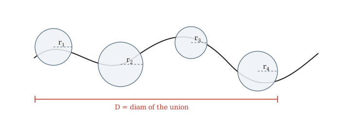
So a family of disjoint balls whose radii sum is large compared to the diameter of their union is a contradiction certificate: it says that the density hypothesis and straightness cannot both hold. The natural quantity to maximize is therefore the score
\[\mathcal{S}_s=\sum_i r_i-\frac{D}{2s},\qquad D=\operatorname{diam}\Bigl(\bigcup_i \overline{B}(x_i,r_i)\Bigr),\]and the question becomes a finite one: for which $s$ does every configuration of centres admit a choice of radii with nonnegative score?
The one place my proof differs from Preiss and Tišer: two colours
This is the point I most want to get across, so let me isolate it.
Preiss and Tišer work with one set. Every ball in their configuration counts mass from the same measure, so every ball must be disjoint from every other ball. That is a severe constraint, and it is what caps their method: the best threshold obtainable from a one-colour argument of that shape is the positive root of $8s^3+4s^2-3s-3$, namely $0.72655\ldots$, and no amount of cleverness inside that framework goes below it.
The pair condition, though, hands you two sets, $E_1$ and $E_2$, and they are disjoint. So colour the centres: red ones will count the mass of $E_1$, blue ones the mass of $E_2$. Two red balls still have to be disjoint from each other, and two blue balls from each other. But a red ball and a blue ball may overlap freely, because the mass counted in a red ball and the mass counted in a blue ball is different mass, and the inequality above still adds up correctly.
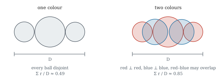
That single relaxation is where the improvement comes from. For the same diameter $D$, letting red and blue interleave lets $\sum_i r_i$ be much larger than any one-colour packing could manage, so the contradiction certificates are far stronger. It is also the entire source of the difficulty: the feasible set is no longer a simple packing region, and the optimization problem that results is genuinely nasty. The structural idea of routing everything through finite optimization problems of this kind is due to De Lellis, Glaudo, Massaccesi and Vittone, and my work solves a particular instance of the family they introduced.
Six points, and why not fewer
The instance I solve uses two colours and three centres of each colour: a root, and two children. Six points in all.
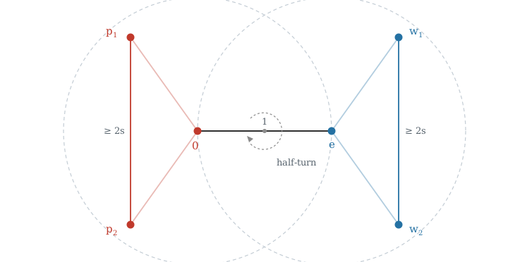
Normalize so that the two roots — the approximate closest points of $E_1$ and $E_2$ — are at distance $1$. Straightness then supplies the children: mass in a ball of radius $1$ whose density is bounded below cannot be concentrated near a single point, so it has to spread, and in a set of finite length spreading means two points at a definite separation. Concretely, each colour gets a sibling pair: two points at distance at least $2s$ from each other, each within distance $1$ of its own root.
Why exactly six? With one centre per colour the problem is trivial and gives nothing. With two, you recover essentially the two-point estimates that underlie the classical bounds. Three per colour is the first count at which the geometry has room to express a real competition, and the competition is what produces a new number. Three families of moves fight each other:
- use only the four children, which is strong when both sibling pairs are long and the cross-colour distances are large;
- use one colour’s two children against all three centres of the other colour;
- use a root together with one of its children against all three centres of the other colour.
Each can be defeated on its own. The content is that defeating one strengthens another: pulling the children in to shorten the cross distances helps the edge-against-triangle moves, and spreading them out helps the four-children move. The optimal constant is the balance point where all three pressures are simultaneously neutral — a nonsmooth optimum where several active constraints meet, not a smooth critical point of a single function. That is why the answer is an algebraic number of high degree rather than something round.
The extremal configuration turns out to be a half-turn: the blue centres are the images of the red ones under rotation by $\pi$ about the midpoint of the two roots, with both red children on the far side of their own root. That symmetry is not assumed; it is derived.
And then it becomes an optimization problem
Once the failure of all the relevant packings is assumed, a finite tree of elementary case distinctions reduces the entire hypothesis to three scalar inequalities, and an algebraic identity turns those into a single weighted score which is forced to be positive. To get a contradiction one has to bound that same score above — and that is a global inequality for two chords in the unit disk, in several variables, which is where all the computation lives.
I am going to leave the details out, because they are not illuminating. The honest summary is that the problem reduces to computationally heavy optimization problems, and that this is precisely the sort of thing an AI can get an approximate solution to by a pile of boring tricks: search the parameter space numerically, round the answer to rationals with a small denominator, and check whether the rounded version still works. What matters is that none of that enters the proof. The parameters found by search are stored as exact rationals; Lean recomputes every downstream coefficient from them in exact rational arithmetic and verifies the sign conditions itself. The key positivity fact is proved as a theorem from an explicit rank-one decomposition, not tested numerically. A search that returns a bad parameter costs time; it cannot make a false statement pass.
Thirty such certificates, covering thirty rectangles of radii, are what close the argument.
Why $0.6934$, and not the sharp constant
The finite six-point problem has an exact optimal constant,
\[\theta_6=s_*=0.693306421825904872690678414403710951\ldots,\]an algebraic number pinned by two radical equations inside an explicit rational box. What I proved is $9.36\times 10^{-5}$ above it. That gap is not a gap in the mathematics; it is the price of making the certificates finite.
At $s_*$ the extremal configuration is attained, and all three packing mechanisms tie there simultaneously. The score I need to bound above by zero is therefore exactly zero at an interior point, with vanishing gradient. Any certificate for a non-strict bound at a degenerate maximum has to resolve the geometry to the precision of the degeneracy, and this is what killed the first fifteen hours: the subdivision needed near the tie grew without bound, and on one coordinate chart the score is identically zero at the extremiser, so no strict certificate of that shape exists there at all.
Moving the chord to the rational value $c=3467/2500$, so that $s=c/2=0.6934$, breaks all three ties at once. The extremal configuration becomes infeasible and the score acquires a uniform negative margin of about $5.8\times 10^{-4}$ — four orders of magnitude more room. That is what lets a small, fixed family of thirty certificates replace an unbounded adaptive search.
Remark: the constant is also bounded from above, which is why it is $0.6934$ and not, say, $0.699$. The separators that prune the case tree are themselves inequalities in the chord, and they fail once $c$ exceeds about $1.386850$. So the admissible window is narrow — above $2s_*$ to break the tie, below that ceiling to keep the pruning — and $6934/10000$ sits inside it.
What comes next
The obvious direction is more points. Six is the smallest count at which the competition described above exists, but there is no reason to stop there: putting more points into each colour’s configuration gives the packing moves more room, which should push the optimal constant of the finite problem down further. The cost is that there are more, and larger, optimization problems to solve, and each one has to end in certificates cheap enough for a kernel to check.
I expect to be able to lower the constant this way, and I will update this post when I do.
I should be clear about the limit, though. Every bound obtained by this route is bounded below by the optimal constant of whatever finite problem it solves, and the six-point method cannot go below $\theta_6$ no matter how cleverly it is certified. Getting to $1/2$ is a different problem. Besicovitch’s conjecture remains open, and nothing here says anything about it.
Links. The repository is CoolRmal/Besicovitchs-1-2; it contains the Lean development, a short paper describing the argument, and an accounting of exactly how much machine time and how many tokens the thing cost. The registry is Palomar, and submissions go through submit.palomar-registry.org. The structural framework is due to De Lellis, Glaudo, Massaccesi and Vittone; the account of Besicovitch’s example that the lower bound follows is Capdevila’s.